Reproducible reports with Jupyter

Authors: Parisa Gregg & Myles Mitchell

Published: September 21, 2023

Jupyter notebooks are a useful tool for Python users of all levels. They allow us to mix together plain text (formatted as Markdown) with Python code. This is beneficial for beginners and experienced data scientists alike:

Beginners that are learning Python for the first time can use Markdown cells to annotate code and record notes.
By splitting up their code into chunks, developers can write and test their code in a modular manner.
Jupyter notebooks are open-source and a convenient format for developers to share reports containing live code, equations, visualisations and narrative text with colleagues.

In this post, we will go deeper with these ideas and show you how to create reproducible HTML and PDF reports with Jupyter. This blog is a follow-up to Quarto for the Python user, which explained how to generate reproducible reports from plain text files with Quarto.

What is Quarto?

Quarto is a free-to-use, open-source software based on Pandoc that enables users to convert plain text files into a range of formats, including PDF, HTML and powerpoint presentations. These documents can contain a mixture of narrative text, Python code, and figures that are dynamically generated by the embedded code.

This has many use-cases:

Your company may have a weekly board meeting to go over the latest sales figures. By having a Quarto presentation that pulls in the latest company sales data, you can regenerate the presentation slides each week at the click of a button.
As a researcher you may be preparing a report for publication. By having the code that generates data tables and figures embedded within the report, regenerating the draft as the experimental data floods in is a breeze!

In our recent blog post, Quarto for the Python user, we used Quarto to render dynamic reports that mix together Python code and narrative text. We used Quarto’s standard workflow, which starts from plain text .qmd files. In this post we will extend these ideas to Jupyter Notebooks.

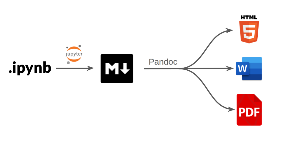
Starting with .ipynb notebook files, the Quarto workflow is:

A flow chart of the Quarto rendering workflow: The ipynb file is first converted to Markdown, with Jupyter used to interpret the code cells. The Markdown file can then be converted to a variety of formats, including HTML, DOCX and PDF, using Pandoc.

A Jupyter kernel is used to interpret the Python code cells and Quarto generates a Markdown document.
The Markdown document includes the text, code, and any figures or results that were generated by the code.
This is then converted into the desired output format (PDF, HTML, etc) using Pandoc.

Prerequisites

We will be using VS Code to edit and render our Jupyter notebook (the only other IDE with support for both Jupyter and Quarto is JupyterLab). Before you can work with Jupyter in VS Code, you will need to install the Jupyter extension. This can be located in VS Code by clicking “Settings” -> “Extensions” then typing “jupyter” into the extensions search bar. Select the “Jupyter” extension by Microsoft and click “Install”.

You will also need to install Quarto. You can then find the Quarto extension in VS Code by typing “quarto” into the extensions search bar. Select the “Quarto” extension and click “Install”.

Finally, to reproduce the examples covered in this post, you will need to install the Python dependencies by running the following command from your terminal:

python3 -m pip install ipykernel nbclient nbformat pandas papermill plotly statsmodels

These dependencies are required for creating an interactive Plotly figure in Jupyter and rendering the notebook from the command line.

Setting up a virtual environment

In case you’d like to follow along with these examples using a virtual environment, we will provide brief instructions for setting up a kernel on Jupyter. If you’re happy to just use your system Python installation then you can move onto the next section.

To create a virtual environment, run the following command from your command terminal:

python3 -m venv venv

This will create a folder called “venv” which can be used to activate the virtual environment (you can call it whatever you like). To activate it, run:

source venv/bin/activate

Now install the Python dependencies into your environment by running the pip command shared above. You can now add this environment to your list of Jupyter kernels by running:

ipython kernel install --user --name=venv

This will add a kernel called “venv”. Next time you open a Jupyter notebook, you should now be able to select this kernel from the list of options.

Rendering a report

We will generate a report about Mario Kart 64 world records. Please refer to our previous post for a recap of the YAML header, Markdown syntax and code chunk options (we will only briefly cover these topics here).

Setting up Jupyter

Within VS Code, create a Jupyter notebook by clicking “File” -> “New File…” -> “Jupyter Notebook (.ipynb support)”. Within the notebook, you can select the kernel by clicking “Select Kernel” and choosing an option from the available list (for example, your system Python installation or a virtual environment). For this post, we used Python 3.10.

Header settings

The first code cell should be changed to a Raw NB Convert cell. In VS Code, the cell type can be changed by clicking the text in the bottom-right corner of the cell (this will read “Python” for a Python code cell). To select a raw cell, type “raw” in the search bar and click the option that appears.

The raw NB convert cell acts as the YAML header of the Quarto report. This is where we include settings such as the title and default output format. Our example is given below:

---
title: "Reporting on Mario Kart 64 World Records"
author: "Parisa Gregg & Myles Mitchell"
date: "1 Aug 2023"
format: html
execute:
    eval: true
jupyter: python3
---

This sets the default output format to HTML and ensures that the code cells are evaluated on execution. Remember to include the fencing (---) for YAML code.

Adding text and code

The remainder of the report will be built from a mixture of Markdown and Python code cells:

Markdown cells are used for narrative text in the report.
Python cells are used for displaying Python code and generating dynamic content (e.g., figures, tables and inline results).

Try copying the following into a Markdown code cell. This adds the Abstract, Introduction and the beginning of the Methods section:

## Abstract

Investigating how the world record for Rainbow Road in Mario Kart 64
developed over time.

## Introduction

Mario Kart 64 is a racing video game developed and published by
[Nintendo](https://en.wikipedia.org/wiki/Nintendo) for the
[Nintendo 64](https://en.wikipedia.org/wiki/Nintendo_64).

Players can choose from eight characters to race as, including:

- Mario
- Toad
- Princess Peach

The game consists of 16 tracks to race around. World records can be
set for either one lap or a full race (three laps) of the course. As
players have competed for faster times, several track shortcuts have
been discovered. There are separate world records for both _with_ and
_without_ the use of a shortcut.

## Methods

We loaded a dataset of [Mario Kart 64](https://mkwrs.com/) world
records. This data is from [tidytuesday](https://github.com/rfordatascience/tidytuesday/blob/master/data/2021/2021-05-25/readme.md)
with credit to [Benedikt Claus](https://github.com/benediktclaus).

For this investigation we are interested in the world records for
Rainbow Road over a three-lap course. The dataset was loaded and
filtered using pandas:

By running the Markdown cell, the text will be rendered so it includes subheadings, bullet points, italic text fomatting and hyperlinks.

Next we may wish to display the code used for loading and filtering the data. Try copying this code into a Python cell:

import pandas as pd

# Load the records data
records = pd.read_csv(
    "https://raw.githubusercontent.com/rfordatascience/tidytuesday/master/data/2021/2021-05-25/records.csv"
)
# Filter the data
rainbow_road = records.loc[
        (records["track"] == "Rainbow Road") &
        (records["type"] == "Three Lap")
].reset_index()
# View the data
rainbow_road.head()

Running this should produce the expected Pandas output, including the first five rows of the rainbow_road data.

Let’s now include some results, starting with a Markdown cell to add the Results section header and opening text:

## Results

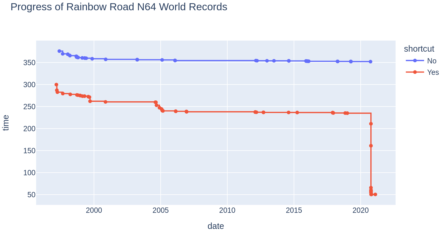
The figure below shows the development of world records for the Rainbow Road
track on Mario Kart 64 from 1997 to 2021.

We could insert the figure as a PNG or PDF image. But to make this report reproducible, let’s dynamically generate the figure using a Python code cell:

#| echo: false
#| fig-cap: "Progress of Rainbow Road world records, with and without allowing shortcuts."
#| fig-width: 8
#| label: wr-plot
import plotly.express as px

px.line(
    rainbow_road,
    x="date",
    y="time",
    color="shortcut",
    title="Progress of Rainbow Road N64 World Records",
    line_shape="hv",
    markers="."
)

The code chunk options at the top of this cell will make the code invisible in the rendered document and set the figure caption, width, and label to our liking. Plotly is used to visualise the world record for Rainbow Road over time. Try running this code within your notebook to check that it generates a figure like the one below:

Image of the plot generated by the Plotly code above. The three-lap world record time is plotted against date from 1997 to 2021. Two coloured lines are shown: red for world records with a shortcut, and blue for without a shortcut.

Finally, let’s quote the longest time a world record was held for using inline code. Copy this code into a Python cell:

#| echo: false
from IPython.display import display, Markdown

max_duration = rainbow_road.record_duration.max()
display(Markdown(
f"""
The longest a 3 lap world record was held 
for on Rainbow Road is {max_duration} days
({round(max_duration/365,1)} years).
"""
))

Running this should add the sentence “The longest a 3 lap world record was held for on Rainbow Road is 2214 days (6.1 years).”, where the numbers 2214 and 6.1 have been calculated by Python. If more data is added, these numbers can be updated automatically by re-rendering the notebook.

Rendering your notebook

You should now have a complete notebook with a YAML header, Markdown text and Python code cells. To see how it should look, you can view our notebook here.

To render the report from the command line:

quarto render <notebook>.ipynb --to html will render the document as HTML.
quarto preview <notebook>.ipynb will generate a live preview which can be viewed as you edit the notebook.
quarto render <notebook>.ipynb --execute will execute the code cells as the output is generated. Without this, you will need to ensure that you have run the code cells in the notebook manually, before quarto is used to render it.

Upon rendering, an HTML document like the one here should be created.

It’s also possible to render the notebook with the VS Code UI. Provided you have the Quarto extension installed, there should be options to “Render”, “Render All”, “Render HTML”, “Render PDF”, and “Render DOCX”:

Screenshot displaying the render options in the VS Code UI. The options are accessed by clicking on the symbol with three dots found in the tool bar. The rendering options include “Render”, “Render All”, “Render DOCX”, “Render HTML” and “Render PDF”.

Note that the HTML plot generated by Plotly cannot be displayed in a DOCX or PDF document. Instead we would have to use a static image format like PNG or PDF.

Cell embedding

In Quarto 1.3 a new feature was added that enables you to embed external Jupyter notebook cells in a Quarto document. This is particularly useful if you have results from different notebooks that you want to extract into a report.

As well as investigating the word records set on Rainbow Road, we have also been looking at those set on Choco Mountain. The results for Choco Mountain are in a separate choco_mountain.ipynb notebook. We might now want to summarise our various Mario Kart results in a single .qmd report (see our previous post for a guide to .qmd reports).

Rather than having to replicate our plotting code, we can embed the relevant cells from our rainbow_road.ipynb and choco_mountain.ipynb notebooks directly into the .qmd report:

---
title: "Reporting on Mario Kart 64 World Records"
author: "Myles Mitchell & Parisa Gregg"
date: "14 June 2023"
format: html
---

## Rainbow Road

The figure below shows the development of world records for the
Rainbow Road track on Mario Kart 64 from 1997 to 2021.

{{< embed rainbow_road.ipynb#wr-plot >}}


## Choco Mountain

The figure below shows the development of world records for the
Choco Mountain track on Mario Kart 64 from 1997 to 2021.

{{< embed choco_mountain.ipynb#wr-plot >}}

Here we have used the “wr-plot” label to reference the code cells that produce the Plotly figures in the Rainbow Road and Choco Mountain reports. These code cells are now embedded in the .qmd report and the figures will be visible in the rendered document (as can be seen here).

Parameterised Reports

Above we produced a report for the Rainbow Road world records on Mario Kart 64. There are 16 tracks in total in the game. What if we wanted to replicate this report for each track? With Quarto and Jupyter notebooks we can define a set of parameters to easily create different variations of a report.

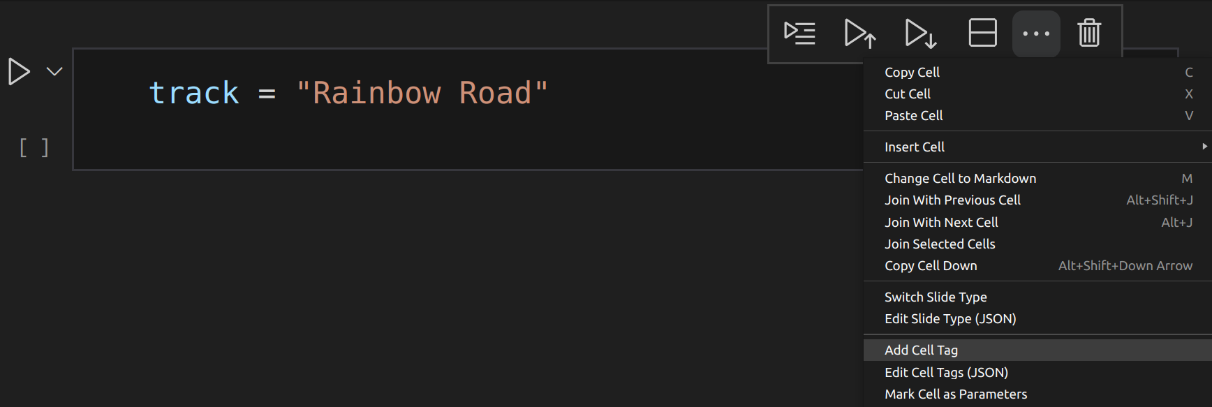
To parameterise a Jupyter notebook we need to create a cell with a “parameters” tag. To add a parameters tag to a Python cell in VS Code, click on “…” (More Actions) in the cell tool bar and select “Add Cell Tag”:

Screenshot depicting how to add a tag to a notebook cell. The cell actions are expanded by clicking on the symbol with three dots in the cell tool bar. The “Add Cell Tag” option is visible in the dropdown list.

To add a parameters tag we then just type “parameters” into the pop up box:

Screenshot showing the pop up box that appears after selecting the “Add Cell Tag” option. A parameters tag is added by typing “parameters” into the box and pressing Enter.

The cell should now have a “parameters” tag:

Screenshot showing a code cell after it has been assigned a parameters tag. A “parameters” label is now visible at the lower-left corner of the cell, with an option to add another tag to the right of it.

If we want to have the track as a parameter in the report, we can define a track variable in the tagged cell (as above):

track = "Rainbow Road"

We can then use this variable in the remainder of our notebook. For example, it can be used to set the track filter in the data-loading code:

# Load the records data
records = pd.read_csv(
    "https://raw.githubusercontent.com/rfordatascience/tidytuesday/master/data/2021/2021-05-25/records.csv"
)
# Filter the data
course_records = records.loc[
        (records["track"] == track) &
        (records["type"] == "Three Lap")
].reset_index()

The full code for our parameterised mario_kart.ipynb notebook can be found here. In this example we have used "Rainbow Road" as the default value for our track parameter. Running the following will therefore generate a report for Rainbow Road:

quarto render mario_kart.ipynb --execute

If we want to report on the "Moo Moo Farm" world records instead, we can pass this to the track parameter on the command line using the -P flag:

quarto render mario_kart.ipynb -P track:"Moo Moo Farm" --execute

You may have noticed that running the above command actually inserts a cell defining the track variable as “Moo Moo Farm” into mario_kart.ipynb.

# Injected Parameters
track = "Moo Moo Farm"