Why should I use R: The Excel R Data Wrangling comparison: Part 1

This is part 1 of an ongoing series on why you should use R. Future blogs will be linked here as they are released.
- Part 1: Why should I use R: The Excel R Data Wrangling comparison: Part 1 (This post)
- Part 2: Why should I use R: The Excel R plotting comparison: Part 2
- Part 3: Why should I use R: Handling Dates in R and Excel: Part 3
The era of data manipulation and analysis using programming languages has arrived. But it can be tough to find the time and the right resources to fully switch over from more manual, time-consuming solutions, such as Excel. In this blog we will show a comparison between Excel and R to get you started!
When choosing between R and Excel, it is important to understand how both solutions can get you the results you need. However, one can make it an easy, reputable, convenient process, whereas the other can make it an extremely frustrating, time-consuming process prone to human errors.
R and Excel
When opening Excel and applying data manipulation techniques to your data, are you easily able to tell what manipulations have been made without clicking on the column or cells? If you were to share these Excel sheets with colleagues are they easily able to replicate your analyses without you telling them where to click or which formulas were applied?
With R all of these are possible. You automatically have all the code visible and in front of you in the form of scripts. Reading and understanding the code is possible because of its easy-to-use, easy-to-read syntax which allows you to track what the code is doing without having to be concerned about any hidden functions or modifications happening in the background.
Most people already learned the basics of Microsoft Excel in school. Once the data has been imported into an Excel sheet, using a point-and-click technique we can easily create basic graphs and charts. R, on the other hand, is a programming language with a steeper learning curve. It will take at most two weeks to become familiar with the basics of the language and the RStudio user interface. Luckily using R can easily become second-nature with practice.
Replicating Analysis
R, while having a slightly steep learning curve, has the ability to reproduce analyses repeatedly and with different data sets. This is very helpful for large projects containing multiple data sets as it keeps our processes clean and consistent. Excel however, because of the point-and-click interface, allows us to rely frequently on memory and repetition, so we would have to repeat the same analyses multiple times by either copying and pasting or simply repeating the point-and-click process, which can be time-consuming, messy, and prone to human errors.
Unlike Excel, R is completely free and benefits from a large community of open-source contributors. To install R and the IDE (RStudio Desktop) to work with R, download and install the relevant versions for your operating system. Once you have successfully installed the IDE, the following user interface will be visible
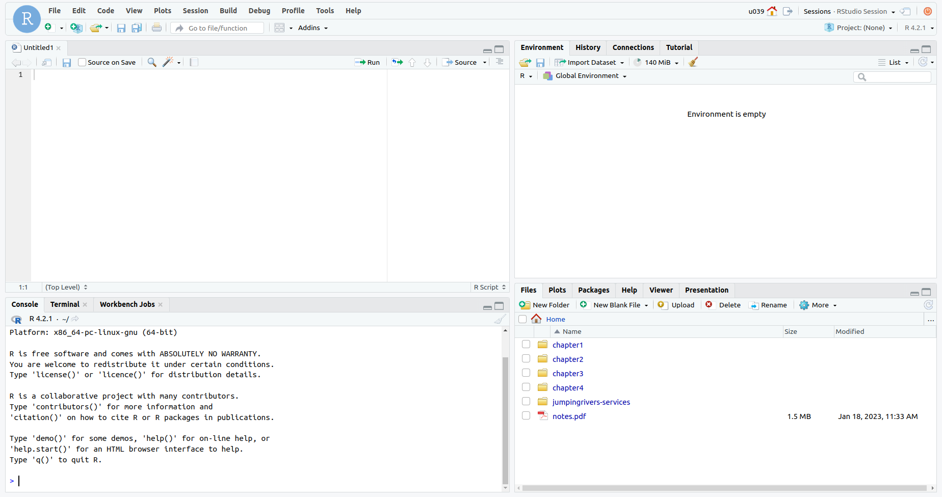
The area on the left is where you will write R code in scripts, use terminals and run jobs. The right hand side of the IDE is comprised of two sections. The top is the environment that stores a list of defined variables and data sets, view the history, and connect to other database. The area below contains five different tabs: the Files tab which lists all of the folders within this project, the Plots tab, which displays any plots that have been generated; the Packages tab which allows you to manage packages within your environment; the Help tab which provides a manual; and the Viewer tab which allows you to view generated interactive content.
Loading the data sets
Excel
The data import steps in Excel are quite straightforward to a day-to-day Excel user, however, it is certainly not reproducible.
Steps:
Click the Data tab on the Ribbon
Click the Get Data button
Select From File
Select from TEXT/CSV
Select the file and click Import
Click Load
R
There are various ways to import data sets such as local files, online
datasets and even through database connections. We will use the
read_csv() function from the {readr} package to import our csv files.
But first, what are packages? R packages are a collection of R
functions, compiled code and sample data that can be installed by R
users. Before using an R function such as read_csv() to import the
data, we are required to install and load the {readr} package. Packages
are great because rather than having to have a huge programme containing
everything you could possibly need, the different packages specialise in
different things, and can be loaded in as and when you need them, saving
a lot of space.
# Installing the package
install.packages("readr")
# Loading the package
library("readr")
# Importing the data
movies_data = read_csv("https://jumpingrivers.com/blog/comparing-r-excel-data-wrangling/movies.csv")
Exploring our data
Before getting started with any data manipulation, let’s explore our data.
Excel
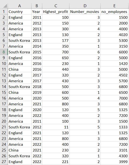
Excel has one basic data structure, which is the cell. These Excel cells are extremely flexible as they store data of various types (numeric, logical and characters). To obtain an overview of the data we could simply just scroll through the Excel data sheet. Now, let’s imagine a data set of 1 million rows and 200 columns, would it still be as easy to scroll through the data sheet to obtain an overview of data? Could we quickly and reliably view all the column names? To me, manually scrolling seems like a very time consuming, unreliable and messy process.
R
To view our data in R, we could simply click on it in the environment or
we could call the name of the data set in the script. If we are working
with a large data set, we can also view a subset of this data by using
functions like head() and tail(). We could also use the colnames()
function to programmatically display the variable names within our data.
movies_data
## # A tibble: 26 × 5
##   Country  Year Highest_profit Number_movies no_employees
##   <chr>   <dbl>          <dbl>         <dbl>        <dbl>
## 1 England  2011            100             3         1500
## 2 America  2012            150             2         2000
## 3 America  2013            300             4         4000
## 4 England  2013            130             2         4020
## # ℹ 22 more rows
str(movies_data) # Displays the structure of the data
## spc_tbl_ [26 × 5] (S3: spec_tbl_df/tbl_df/tbl/data.frame)
##  $ Country       : chr [1:26] "England" "America" "America" "England" ...
##  $ Year          : num [1:26] 2011 2012 2013 2013 2013 ...
##  $ Highest_profit: num [1:26] 100 150 300 130 177 350 700 650 230 440 ...
##  $ Number_movies : num [1:26] 3 2 4 2 3 1 6 2 1 3 ...
##  $ no_employees  : num [1:26] 1500 2000 4000 4020 5300 3150 6000 5000 1420 5000 ...
##  - attr(*, "spec")=
##   .. cols(
##   ..   Country = col_character(),
##   ..   Year = col_double(),
##   ..   Highest_profit = col_double(),
##   ..   Number_movies = col_double(),
##   ..   no_employees = col_double()
##   .. )
##  - attr(*, "problems")=<externalptr>
head(movies_data) # Displays the first six rows of the data
## # A tibble: 6 × 5
##   Country  Year Highest_profit Number_movies no_employees
##   <chr>   <dbl>          <dbl>         <dbl>        <dbl>
## 1 England  2011            100             3         1500
## 2 America  2012            150             2         2000
## 3 America  2013            300             4         4000
## 4 England  2013            130             2         4020
## # ℹ 2 more rows
tail(movies_data) # Displays the last six rows of data
## # A tibble: 6 × 5
##   Country  Year Highest_profit Number_movies no_employees
##   <chr>   <dbl>          <dbl>         <dbl>        <dbl>
## 1 England  2021            120             1         1325
## 2 America  2021            800             3         6800
## 3 America  2022            400             2         7200
## 4 China    2021            230             2         3101
## # ℹ 2 more rows
colnames(movies_data) # Displays all the variable names
## [1] "Country"        "Year"           "Highest_profit"
## [4] "Number_movies"  "no_employees"
The movies data is comprised of five columns: country, year, highest
profit gained per movie, number of movies produced and number of
employees on set during production. It is clear that R programmatically
displays the output of our data whereas Excel requires of a lot of
eye-balling and manual scrolling. If we were interested in displaying a
subset of our data, in a report for example, using R we could simply use
the functions above. To do this in Excel we would have to copy and paste
the first 6 rows of the data and manually add it to the report document.
Summary Statistics
Now, let’s apply some summary statistics on our data. Summary statistics provide a quick summary of data and are particularly useful for comparing one project to another, or before and after.
Excel
It is very well known that Excel has a data storage limitation per spreadsheet. It can have a very limited amount of columns and rows, while R is made to handle larger data sets. Excel files are also known to crash when they exceed 20 tabs of data. Excel is able to handle a good chunk of data, but not much. This becomes very risky when you unknowingly start to lose data because the file has become too big and is unable to save. To generate summary statistics (such as the minimum and maximum values) of our data in Excel, we followed a few steps:
Scroll to the Home tab
In the Editing group, click the arrow next to AutoSum
Click Min
Click Max
Press Enter
These steps were quite easy to follow, however, I often forget where to click or which tab to select. After discussing this workflow with a colleague, we also discovered slight differences in the steps for different versions of Excel. This did not seem very effective or reproducible to us.
R
summary(movies_data)
##    Country               Year      Highest_profit
##  Length:26          Min.   :2011   Min.   : 11
##  Class :character   1st Qu.:2013   1st Qu.:157
##  Mode  :character   Median :2017   Median :320
##                     Mean   :2017   Mean   :350
##                     3rd Qu.:2021   3rd Qu.:485
##                     Max.   :2022   Max.   :800
##  Number_movies   no_employees
##  Min.   :1.00   Min.   :1325
##  1st Qu.:2.00   1st Qu.:2275
##  Median :2.50   Median :4401
##  Mean   :2.65   Mean   :4338
##  3rd Qu.:3.00   3rd Qu.:6375
##  Max.   :6.00   Max.   :7200
# Stardard deviation
sd(movies_data$Highest_profit)
## [1] 224
# Highest value of the Highest profit column
min(movies_data$Highest_profit)
## [1] 11
# Highest value of the Highest profit column
max(movies_data$Highest_profit)
## [1] 800
The dollar symbol, $, used here simply dictates which data set and
column we are using for the analysis. It is evident that the source code
of R can be used repeatedly and with different data sets in ways that
Excel formulas cannot. R clearly shows the code (instructions), data and
columns used for an analysis in ways that Excel does not. If I were to
share this script with a colleague they would have a complete
understanding on how the summary statistics were generated because of
R’s human readable syntax.
Data Wrangling
Data manipulation tools assist us with modifying our data to make it easier to read and organise. For example, one of the easiest data manipulation tools in Excel is inserting columns and rows. The purpose of data manipulation is to create a consistent, organised and clean data set. With this in mind, let’s apply the following data manipulations in Excel and then R:
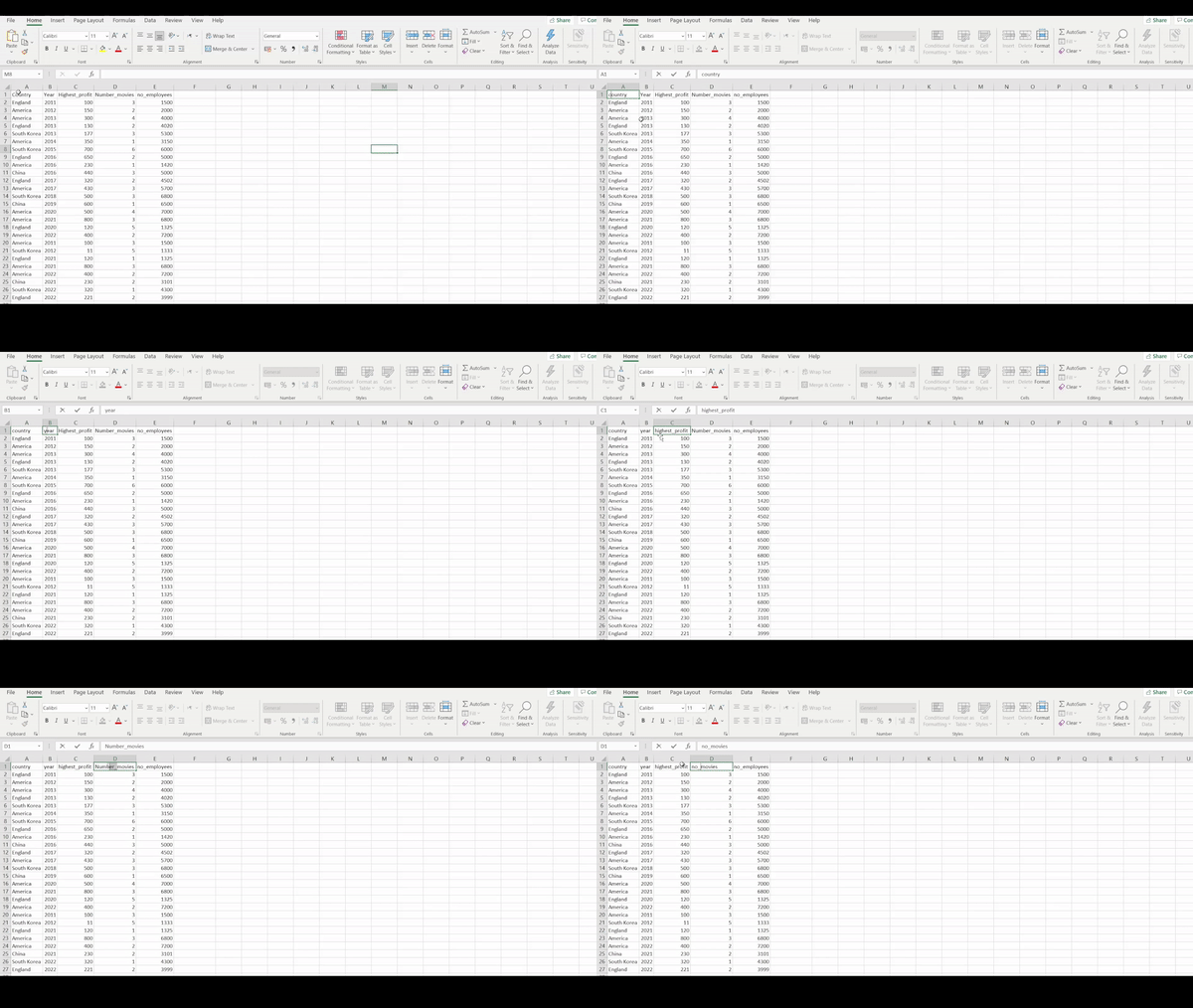
- Rename the columns into a consistent format
- Arrange the year column in ascending order
- Select and create a new column
- Remove a column from the data
- Select only the entries for the year 2014
- Remove only the entries from rows 4-11
1. Renaming columns in R and Excel
Excel
Renaming columns in R is a completely manual process, which makes it an extremely time-consuming and risky process especially if you are working between multiple messy Excel sheets.
R
For data manipulation in R, we use a powerful package in R called {dplyr}. Let’s load and install the package.
# Installing the packages
install.packages("dplyr")
library("dplyr")
To rename the columns, there is a handy function called rename(). We
simply pass this function the name of our data set (movies_data), and
then rename each of the columns. There are other methods available in
other packages which can automatically make everything lower case, for
example, but for the purposes of this blog, we will stick with {dplyr}.
# Renaming the column into a consistent format
movies_data = rename_with(movies_data, tolower)
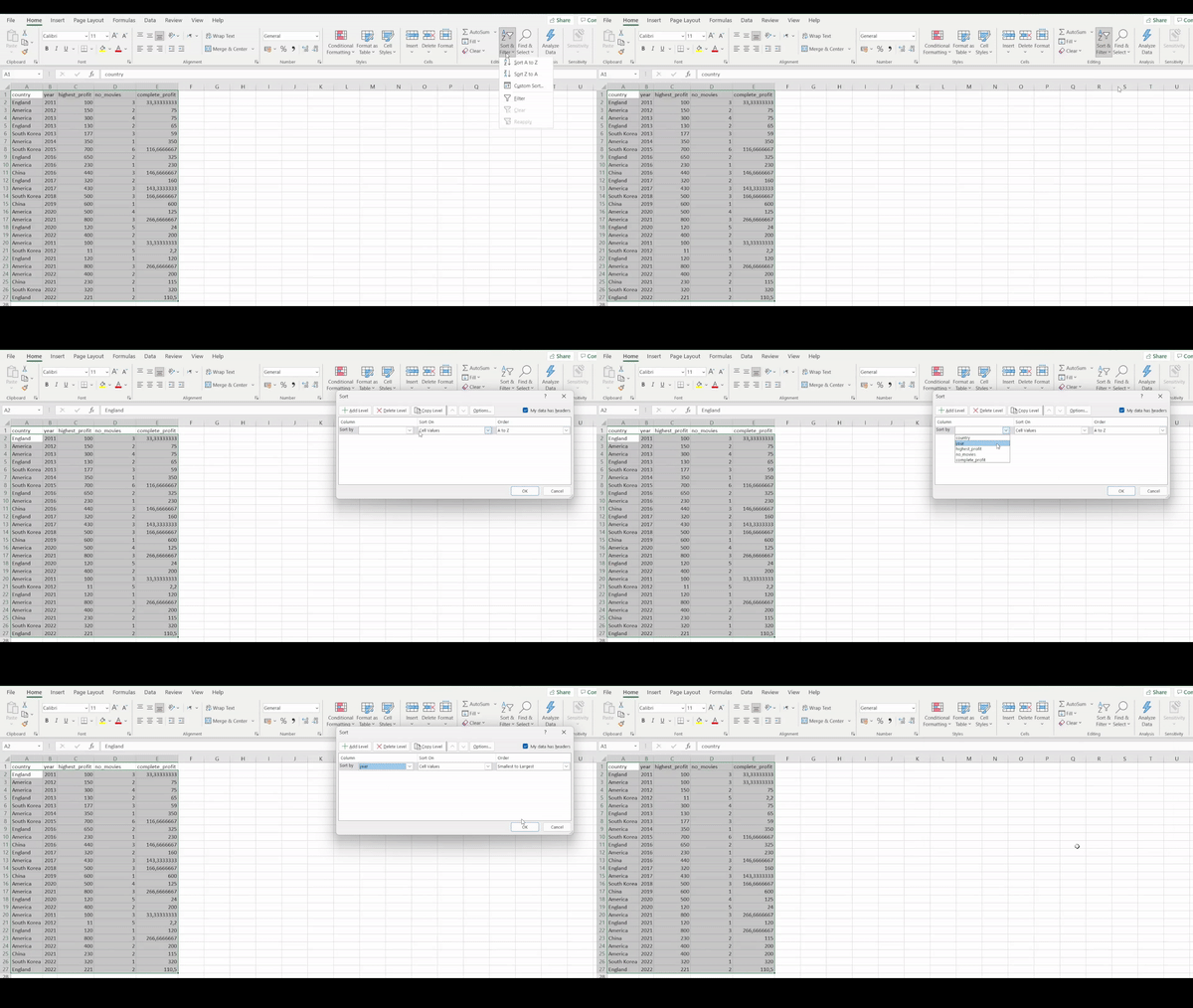
2. Arrange the year column in ascending order
Excel
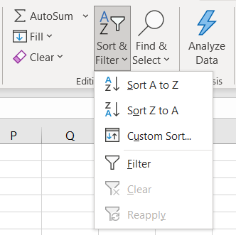
To change column to ascending order, we first had to:
Select the
yearcolumnDirect to the
Sort and Filter tabSelect the option to sort from the largest to the smallest value
R
arrange(movies_data, year)
## # A tibble: 26 × 5
##   country    year highest_profit number_movies no_employees
##   <chr>     <dbl>          <dbl>         <dbl>        <dbl>
## 1 England    2011            100             3         1500
## 2 America    2011            100             3         1500
## 3 America    2012            150             2         2000
## 4 South Ko…  2012             11             5         1333
## # ℹ 22 more rows
Again, with Excel representing a point-and-click nature, it is impossible to identify. by looking at a column, how the data was modified. If I were to replicate these steps in two years time I would likely have forgotten where to point and click. With R however, we have our code which clearly shows each step used to manipulate the data. If I were to return to my script in two years time, I would easily be able to replicate the analysis.
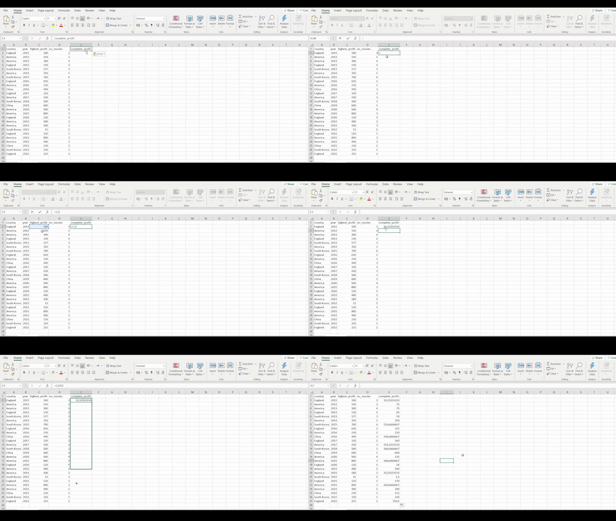
3. Selecting and adding a new column
Let’s reduce our data set by first selecting the country, year,
number_movies and highest_profit columns. Then we will generate a
new column called complete_profit. The complete_profit column should
be generated from taking the highest_profit column divided by the
no_movies column.
Excel
R
movies_data %>%
  select(country, year, number_movies, highest_profit) %>%
  mutate(complete_profit = highest_profit/number_movies)
## # A tibble: 26 × 5
##   country  year number_movies highest_profit
##   <chr>   <dbl>         <dbl>          <dbl>
## 1 England  2011             3            100
## 2 America  2012             2            150
## 3 America  2013             4            300
## 4 England  2013             2            130
## # ℹ 22 more rows
## # ℹ 1 more variable: complete_profit <dbl>
4. Removing a column
Excel
In Excel, inserting or deleting a column is a manual process. First, we select the column then right-click at the top of a column and then select the Delete option.
R
select(movies_data, -year)
## # A tibble: 26 × 4
##   country highest_profit number_movies no_employees
##   <chr>            <dbl>         <dbl>        <dbl>
## 1 England            100             3         1500
## 2 America            150             2         2000
## 3 America            300             4         4000
## 4 England            130             2         4020
## # ℹ 22 more rows
In R, we simply used the select function from the {dplyr} package to
select a column of our data frame. To remove a column we put a - in
front of the variable to exclude it from our data.
5. Select only the entries for a particular year
Excel
Here we are interested in extracting the data collected only during the year 2021. Using Excel software, we first sort the year column and then manually select the years that we are interested in. While applying this manual technique of selecting pieces of data that we are interested in, it is very easy to select the wrong data or even accidentally delete data.
R
filter(movies_data, year == 2021)
## # A tibble: 4 × 5
##   country  year highest_profit number_movies no_employees
##   <chr>   <dbl>          <dbl>         <dbl>        <dbl>
## 1 America  2021            800             3         6800
## 2 England  2021            120             1         1325
## 3 America  2021            800             3         6800
## 4 China    2021            230             2         3101
6. Remove only the row entries from 2-4
Excel
Removing rows in Excel is once again a manual process. We select the rows that we do not want to keep, then right click and delete those rows. These rows are now permanently deleted from the data sheet. If we were interested in adding them back into the sheet, we would have to find it (if we had a back up Excel sheet) and copy and paste it back into our data analysis Excel sheet. If we did not have a back up of the data that we had deleted, then this data would be completely lost.
R
In R we can use the slice() function to return a subset of rows based
on their position. If you want to remove rows using slice() instead of
retaining them you can just add a - in front of the row indices you’re
passing into the function. So, to remove rows 2, 3, and 4:
slice(movies_data, -(2:4))
## # A tibble: 23 × 5
##   country    year highest_profit number_movies no_employees
##   <chr>     <dbl>          <dbl>         <dbl>        <dbl>
## 1 England    2011            100             3         1500
## 2 South Ko…  2013            177             3         5300
## 3 America    2014            350             1         3150
## 4 South Ko…  2015            700             6         6000
## # ℹ 19 more rows
Using R and Excel
There are multiple ways in which data manipulation is used efficiently in data science. Data formatting is important and must be organised to be read by the various software programs, be it in R or Excel.
Excel is an excellent tool and is easy to use and at times it is the most appropriate tool. Excel is often used for data processing work under general and basic office requirements. However, Excel is limiting in that the data file itself can hold only approximately 1 million rows without the aid of other tools. The basic built in statistical analysis is too simple and has very little practical value. If you are an aspiring data analyst, you will need to expand your toolset and start thinking beyond the rows and columns of a spreadsheet. R functions cover almost any area where data is needed. Getting started with R is very simple especially because of the easy-to-use and understandable syntax. Most importantly, R facilitates reproducible analyses.
A hammer is great for driving nails, but it’s not the only tool out there.
If you’re interested in learning R, then attend our Introduction to R course.

